Spline Example: A Modulating Input Function

Summary

In this example, it is demonstrated how a continuous input function that modulates the right-hand side of an ODE in a time-dependent manner can be estimated without direct observations. The model used for demonstration purpose is an SEIR model. These models are frequently applied for describing the dynamics of infection diseases. In this context, the time-dependent modulation originates from political containment actions that reduces the infection rate.

In particular, instead of a common rate or reaction

Susceptibles -> Exposed   CUSTOM "b * Infectious * Susceptibles"	"description"

it might be desired to have a time dependent b, e.g.

Susceptibles -> Exposed     CUSTOM "b * b_time_dependence * Infectious * Susceptibles"	"description"

where b_time_dependence denotes a custom function of time.

The aim of this example is not having a realistic model and a common parametrization from literature. Instead, the model is rather simple for demonstrating capabilities of D2D in input estimation.

The implementation is available in folder Examples/ToyModels/SplineExample_InputModulation

Illustration problem

In the example, the infection rate is known to be time dependent due to containment actions but the functional form is unknown. Moreover, the infection rate is not observed directly. Only the infected people termed as "Infectious" are observed.

Smoothing splines are frequently applied for estimating smooth functional relationships. Splines are polynomials that are defined in intervals and connected at so-called "knots" via boundary conditions that ensure a continuity up to the 2nd derivative.

The shape of a smoothing spline depends on the data and the degrees of freedom, i.e. the number of knots. In our implementation, one knot corresponds to one parameter. In D2D, parametrization is chosen that the parameter depends on the value of the spline at each knot.

In the context of ODE-modelling, one typical challenge of using splines as input functions is that negative values should be prevented. This can be done by using the spline as exponent, i.e. the input that enters to the right hand side of the ODEs is given by 10^spline(t). In the context of this illustration example, the restrictions are even stronger because the spline should be within the range (0,1]. Moreover, it was intended for prediction purpose to switch-off the impact of the smoothing spline after the last observation.

Implementation

Restricting the range of the spline

In our implemenation, the smoothing spline s(t) with 10 knots was linked with a sigmoidal function

f(s) = exp(s)/(1+exp(s))

This function f is zero for small s and one for large s.

In the model definition file, the implementation reads

INPUTS
InputSpline    C   1	1  "spline10(t, 0.0, 5, 10.0, sp2, 20.0, sp3, 30.0, sp4, 40.0, sp5, 50.0, sp6, 60.0, sp7, 80.0, sp8, 150.0, sp9, 400.0, 5, 0, 0.0)"
...

DERIVED
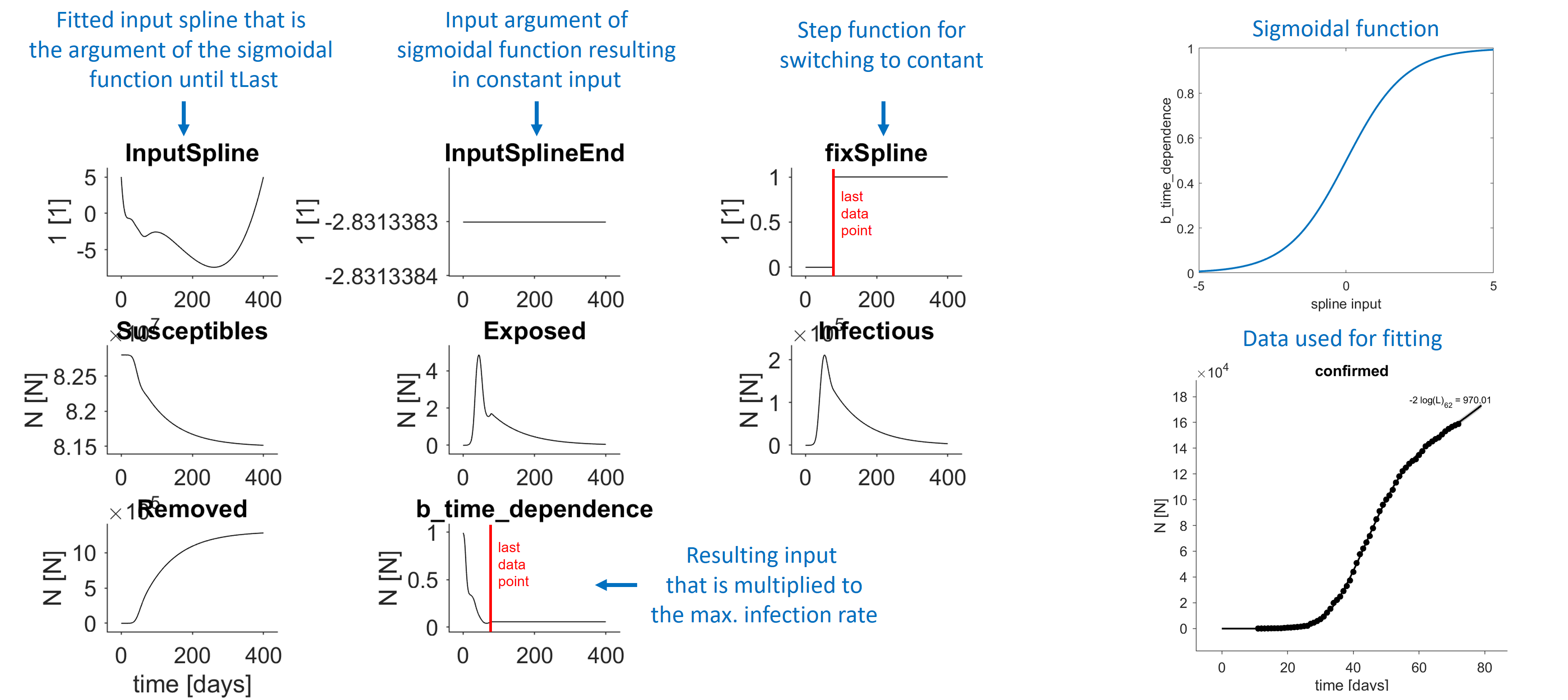
b_time_dependence      C   "N"   "N"   "exp(InputSpline)/(1+exp(InputSpline))"

Note, that the spline has a prespecified number of ten knots, at t=0, 10, 20, 30, 40, 50, 60, 80, 150, 400 but only 8 free parameters. [Alternatively, the time points of the knots could also be implemented as parameters. However, optimization of these knot times is not supported by D2D because it would require intricate derivative computations.] The first and the last spline parameters are set to 5 because f(5) is close to one. This is a further intended constaint of the model.

Switch to constant input

In order to keep the input constant after the last data point, a second spline-input is defined that shares the parameters sp2, ..., sp9. Instead of the model time t, the second spline depends on the argument tLast. This means, that the second spline has the same response as the first for t=tLast. In order to switch from the first to the second spline at t=tLast, both splines are connected with an a step input in the following way:

INPUTS
InputSpline       C  1	1  "spline10(t, 0.0, 5, 10.0, sp2, 20.0, sp3, 30.0, sp4, 40.0, sp5, 50.0, sp6, 60.0, sp7, 80.0, sp8, 150.0, sp9, 400.0, 5, 0, 0.0)"
InputSplineEnd    C  1  1  "spline10(tLast, 0.0, 5, 10.0, sp2, 20.0, sp3, 30.0, sp4, 40.0, sp5, 50.0, sp6, 60.0, sp7, 80.0, sp8, 150.0, sp9, 400.0, 5, 0, 0.0)"
fixSpline         C  1  1  "step1(t, 0, tLast, 1)"
...

DERIVED
b_time_dependence  C   "N"   "N"   "exp(InputSpline)/(1+exp(InputSpline))*(1-fixSpline) + fixSpline*exp(InputSplineEnd)/(1+exp(InputSplineEnd))"

Event times

The last measurement time point of the data can be obtained "manually" in the following way:

tLast = -Inf;
for d=1:length(ar.model.data)
    iy = contains(ar.model.data(d).y,'confirmed');
    notnan = ~isnan(ar.model.data(d).yExp(:,iy));
    tmax = max(ar.model.data(d).tExp(notnan));
    tLast = max(tmax,tLast);
end

For reliable optimization, it is essential to treat the time point where the derivative of the spline input is not continuous (i.e. tLast) as an event. This can be implemented in the following way:

arSetPars('tLast',tLast,0,0,1,100,0);
for c=1:length(ar.model.condition)
    arAddEvent(1,c,tLast);
end

Note: These code lines contain loops over ar.model.data and ar.model.conditions. In the easy example model, these loops can be omitted because there is only a single ar.model.data and a single ar.model.condition.